Image processing
Analysing an image requires that we process it into a desired state.
Point operations
Point operations, like their name operate on only one point (pixel) at once. Some obvious ones that come to mind are brightness, contrast, gamma modifications.
Formally,
If we define an image as a function
Brightness and Contrast
One simple, linear point operation is
Here, a is called the
Contrast stretching
We can model the contrast of an image to scale however we want. Usually with functions that have a high slope in the intermediate intensities, and then slowly taper off at the 0 and maximum intensities.
For visualization, maybe imagine a function like this, takes intensity as input, and gives out intensity for new image.
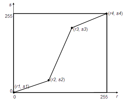
Basically, scale contrast in some other way to highlight the important intensities.
Linear interpolation
Lerping is also a point operation. We linearly interpolate between two target values, with an interpolation parameter
This function, linearly blends between the two functions, with respect to
Lerping can be extended to be non linear by using other polynomial functions as the multipliers for each function.
Gamma correction
Our eyes percieve light non linearly. So, a linear gradient of colors on the screen, say a lerp from white to black, will not appear linear and even to our eyes. So, we create a non linear mapping of colors instead, by gamma correcting, so that when our eyes do their non linear transformation, it cancels out.
In simpler terms, if the human eye applies a transformation
Thresholding
Given a certain threshold, we decide what to do with pixels on either side of the intensity threshold. Some of the common ways to handle these are -
- Binary: Everything below is set to 0, everything above is set to 100%
- To zero: Everything below is set to 0, everything above remains as is
- Clip: Everything above threshold is set to threshold, everything below remains as is
There is one more method that is often used with Canny edge detection which is called hysterisis thresholding. It it not a point operation but is discussed here nevertheless.
In hysterisis thresholding, we have two thresholds - say lower and upper. Anything above upper is considered an edge. And anything below is considered to be not an edge. Anything in between is only considered edge, if adjacent pixel is also edge.
Grayscale
A grayscale image is an image with just one channel, to represent shades of white (or black?). It is as simple as taking the arithmetic mean of all color channels, to generate our grayscale image.
Linear filters
In linear filter, we operate on the function with something called a kernel. It is often called, a mask, a filter, a convolution filter and such. But it is just a matrix that is slided over the given function, and sum of products is calculated
Operations
Correlation
Correlation involved moving the center of a mask (called a kernel), over the image and computing the sum of all products after elementwise multiplication. The values in the kernel are called filter coefficients. The operator for correlation is represented as
The center of the kernel is moved accross the image. For the pixels at the edge, this would mean half the kernel ends up outside the image. So, we pad the image with 0s. For a kernel of size
Convolution
Convolution is correlation, but the kernel is rotated by
Seperable linear filtering
The number of operations for Convolving/correlating a 2D matrix per pixel is a quadratically dependent on the dimensions of the kernel.
But it can be shown that,
any matrix
Where, x is a column vector and y is a row vector.
It can also be shown that the matrix multiplication of a column and row vector is a 2d convolution of those vectors.
And since convolution is commutative;
So, the number of operations is brought down to the number of operations in 2 successive convolutions with a column and row vector, which is linearly dependent on the dimensions of the filter.
Two such important filters that are also seperable are discussed below.
Box filter
A standard box filter, also called a mean filter, consists of a kernel, with all of its elements equal to the dimensional area of the kernel. Convolving with a box filter has the effect of taking average of an area of pixels, therefore producing a blurred image as the output.
This has the unwanted effect of producing box-y artifacts.
Gaussian filter
A Gaussian filter used a 2D Gaussian distribution as the kernel values.
Formally, for a Gaussian filter
Where,
On increasing the variance of the distribution, we also increase the blur effect. This blurring is called Gaussian smoothing, or Gaussian blur.
Seperability of the Gaussian distribution
A 2D Gaussian filter can be seperated into two 1D Gaussian vectors, whose matrix multiplication gives us back the 2D filter.
This allows for significant speedups, for larger kernel sizes.
Non linear filters
With non linear filtering, we still use the concept of kernels and sliding them over an image. But we do not perform linear combination operations with the kernel and the image. We can pick an arbitrary function to decide the output of the non linear filter. Some examples will make it clear.
Median filter
For any given pixel, we center the kernel at that pixel. And then we find the median of all of the image's pixels that fall inside the kernel. The output image is assigned this median pixel. Median filters reduce noise, while also causing blurring that scales with the kernel size.
Bilateral filter
In the Gaussian filter above, we use a Gaussian distribution to populate the values of the kernel, solely based on the coordinates of each cell in the kernel. So, if we refer to that as spatial gaussian, bilateral filtering introduces something called the brightness gaussian.
The brightness gaussian takes as input the difference in intensities of two pixels. The Gaussian distribution, as we know, starts off high near the origin and then smooths out, so if the intensity difference was low (we would be close to the origin), we would get a larger output from the brightness gaussian. If we use the output of the brightness gaussian as the gain for the spatial gaussian (basically if we multiply spatial and brightness gaussians), we end up giving more weight to similar pixels, and lower weight to dissimilar pixels.
As for normalizing the output to
Got confused about why a bilateral filter is non linear. It is because we aren't exactly doing a convolution operation, as the kernel dynamically adapts each time it moves.
Morphological operations
They're called morphological because they focus more on the structure, shape of the image (or a subset of the image) and not directly on the pixel values.
A structuring element (kernel) is scanned over an image, and an output is generate by some selective function. These are generally used on binary images (simplest possible bitmap), but can still be used on other types of images too (some modification might be required, below operations are discussed as generally as possible)
Dilation and Erosion
Dilation and erosion are two morphological function, where the selective function used by the structuring element is maximum and minimum respectively. Clearly
- Dilation adds pixels to boundaries
- Erosion removed (erodes) pixels from boundaries
Opening and Closing
When an image is eroded, noise artifacts are reduced or even removed. Now, on dilation, pixels are only added to boundaries that exist after erosion. So, opening reduces noise.
Similarly, dilation followed by erosion patches up small holes or gaps in an image, by adding pixels first (which might fill said holes) and then eroding pixels from the boundaries.
Morphological gradient
On dilating an image, we sort of "increase" the boundary size. And on erosion, we "decrease" it. It is clear that taking the difference of these two outputs, that is subtracting the eroded image from the dilated image, will yield only the boundary pixels being lit up.
Geometric transformations
Multiplying a matrix can be thought of as applying a linear transformation. A linear transformation could be -
- Translation
- Rotation
- Scaling and stretching
- Any combination of these
Affine transformation
3 non collinear points can be used to describe a plane. For stretching, scaling, rotating or translating this plane, we just need one matrix to apply a transformation (by definition that is matrix multiplication). This affine matrix encodes all information needed to map from a source triangle to a destination triangle. And so all points transformed by it undergo the same transformation as the triangles.
A matrix multiplication is just applying a transformation. Muliplying with a matrix
- The current
- The current
Rotation
So a rotation by
By our earlier perspective about what a matrix is, we can derive a rotation matrix as
Translation
For translation,
Resizing
For resizing an image, we map the pixels according to the scale factor first. And then decide how to fill in the gaps, with whatever interpolation method we want.
Some interpolation methods are discussed below as examples.
Consider a 4x4 image that has to be scaled up to 9x9. The scale factor is calculated as 4x4 image. Now clearly, there is no pixel with indices (0.375, 0.375) in the 4x4 image. So, we can handle this in one of these given ways.
Nearest neighbor
For nearest neighbour, it is pretty simple, we simply round the fractional indices (not floor and nor ceil, but round). And we simply use that pixel's value. This clearly results in pixels being duplicated and jagged edges, but it might be desirable for applications like pixel art.
Bilinear interpolation
Basically the pixel with fractional indices has 4 pixels influencing it (obtained by floor and ceil in all combinations). We lerp between any two pixels first, and then using the result, lerp between the other two.
For example, for (0.375, 0.375) we lerp between the values of pixels at (0, 0) and (1, 0) with 0.375 as parameter, let us call this result A; we also lerp between pixels (0, 1) and (1, 1) and call this result B. We finally lerp between A and B with 0.375 as parameter.
Related: Edge detection